Activation Functions & Optimizers

• Activation Functions
• Gradient Optimizers

Activation Functions

In the following subsections, I will denote $z$ as the input to a neuron and $y$ as the output of the neuron, where $z = w^{T}x + b$, and $w$ is the weights for input $x$, $b$ is the bias.

1. Linear Activation Function
   The output of a linear neuron is linearly dependent on its inputs, which can be expressed as:
   $y = cz;$
   where $c$ is some constant

2. Binary Threshold Activation Function
   In a binary threshold neuron, if the net input to the neuron exceeds a specified threshold then the neuron is activated and outputs 1, otherwise 0. It can be expressed as:
   $y = 1 \;\;\; if \;\; z > k; \\ y = 0 \;\;\; if \;\; z <= k; \\ $
   where $k$ is some threshold.

3. Sigmoid Activation Function
   The input–output relation for a sigmoid neuron is expressed as the following:
   $y=\frac{1}{1+e^{-z}}$
   
   

4. SoftMax Activation Function
   The SoftMax activation function is a generalization of the sigmoid function and is best suited for multi-class classification problems. If there are $k$ output classes, then the predicted probability for the $ith$ class given the input vetor $x \in \mathbb{R} ^{n \times 1}$ is given by the following:
   $P(y_{i}=1/x)=\frac{e^{z_{i}}}{\sum_{j=1}^{k} e^{z_{j}}}$
   when $k$ is 2, the preceding equation is the same as sigmoid activation function.
   
   The loss function for the softnax activation function is called categorical cross entropy and is given by the following:
   $C = \sum_{i=1}^{k}-y_{i}logP(y_{i}=1/x)$
   
   Logistic regression, sigmoid, and softmax are all related to cross entropy, so let’s take a closer look at it. If we have a probability distribution $p$ that is the true distribution, and we have a predicted probability distribution $q$, we can use cross entropy to measure the dissimilarity between $p$ and $q$ by using the preceding equation.
   Take logistic regression as an example, if output $y \in {0,1}$, then $q(y=1)=\frac{1}{1+e^{-z}}=\hat{y}$ and $q(y=0)=1-\hat{y}$. The true probabilities can be expressed similarly as $p(y=1)=y$ and $p(y=0)=1-y$. So, we now have $p\in{y, 1-y}$, and $q\in{\hat{y}, 1-\hat{y}}$, so can use cross entropy to get a measure of dissimilarity between $p$ and $q$:
   $C(p,q)=\sum_{i=1}^{k}-p_{i}logq_{i}=-ylog\hat{y}-(1-y)log(1-\hat{y})$

5. Rectified Linear Unit(ReLU) Activation Function
   In a rectified linear unit, the output equals the net input to the neuron if the overall input is greater than 0; however, if the overall input is less than or equal to 0 the neuron outputs a 0. The output for a ReLU unit can be represented as follows:
   $y = max(0, z)$
   
   
   
   The ReLU is one of the key elements that has revolutionized deep learning. They are easier to compute. ReLUs combine the best of both worlds—they have a constant gradient while the net input is positive and zero gradient elsewhere. If we take the sigmoid activation function, for instance, the gradient of the same is almost zero for very large positive and negative values, and hence the neural network might suffer from a vanishing-gradient problem. This constant gradient for positive net input ensures the gradient-descent algorithm doesn’t stop learning because of a vanishing gradient. At the same time, the zero output for a non positive net input renders non-linearity.
   
   There are several versions of rectified linear unit activation functions such as parametric rectified linear unit (PReLU) and leaky rectified linear unit. For a normal ReLU activation function, the output as well as the gradients are zero for non-positive input values, and so the training can stop because of the zero gradient. For the model to have a non-zero gradient even while the input is negative, PReLU can be useful. The input–output relationship for a PReLU activation function is given by the following:
   $y =max (0,z )+ \beta min(0,z )$
   when $\beta$ is -1, then $y=|z|$ and the activation function is called absolute value ReLU. When $\beta$ is set to some small positive value, typically around 0.01, then the activation function is called leaky ReLU.

6. Tanh Activation Function
   The input–output relationship for a tanh activation function is expressed as:
   $y=\frac{e^{z}-e^{-z}}{e^{z}+e^{-z}}$
   
   
   
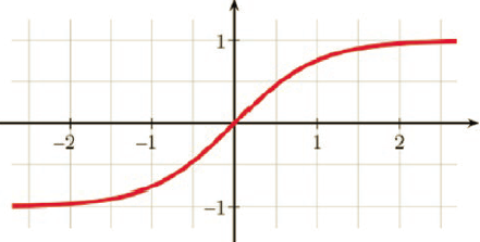
   The sigmoid activation function saturates at around output 0. While training the network, if the outputs in the layer are close to zero the gradient vanishes and training stops. The tanh activation function saturates at -1 and + 1 values for the output and has well-defined gradients at around the 0 value of the output. So, with tanh activation functions such vanishing-gradient problems can be avoided around output 0.

Gradient Optimizers

TensorFlow has a rich inventory of optimizers for optimizing cost functions. The optimizers are all gradient based, along with some special optimizers to handle local minima problems. We shall see what they are about. Before we go into it in details, let’s familiar with some commonly-used terms in deep learning.

• Batch size
  The batch size determines the number of training data points in each mini batch. The batch size should be chosen such that it gives a good enough estimate of the gradient for the full training dataset and at the same time noisy enough to escape bad local minima that don’t provide good generalization.

• Number of batches
  The number of batches gives the total number of mini batches in the entire training dataset. It can be computed by dividing the count of the total training data points by the batch size. Please note that the last mini batch might have a smaller number of data points than the batch size.

• Epochs
  One epoch consists of one full pass of training over the entire dataset. To be more specific, one epoch is equivalent to a forward pass plus one backpropagation over the entire training dataset.

1. GradientDescentOptimizer
   GradientDescentOptimizer implements the fundamental full-batch gradient-descent algorithm and takes the learning rate as an input.

2. AdagradOptimizer
   AdagradOptimizer is a first-order optimizer like gradient descent but with some modifications. Instead of having a global learning rate, the learning rate is normalized for each dimension on which the cost function is dependent. The learning rate in each iteration is the global learning rate divided by the $l^{2}$ norm of the prior gradients up to the current iteration for each dimension.
   
   If we have a cost function $C(\theta)$ where $\theta=[\theta_{1}\theta_{2}\theta_{3}…\theta_{n}]^{T}\in\mathbb{R}^{n\times 1}$, then the update rule for $\theta_{i}$ is as follows:
   $\theta_{i}^{t+1}=\theta_{i}^{t}-\frac{\eta }{\sqrt{\sum_{\tau=1}^{t}\theta_{i,\tau}^2+\varepsilon}}\frac{\partial C^{t}}{\partial \theta_{i}}$
   where $\eta$ is the learning rate and $\theta_{t}$ and $\theta_{t+1}$ are the values for the $ith$ parameter at iterations $t$ and $t +1$ respectively.
   
   Sometimes sparse features that don’t show up much in the data can be very useful to an optimization problem. However, with basic gradient descent or stochastic gradient descent the learning rate gives equal importance to all the features in each iteration. Since the learning rate is same, the overall contribution of non-sparse features would be much more than that of sparse features. Hence, we end up losing critical information from the sparse features. With AdagradOptimizer, each parameter is updated with a different learning rate. The sparser the feature is, the higher its parameter update would be in an iteration. This is because for sparse features the quantity $ \sqrt{\sum_{\tau=1}^{t}\theta_{i,\tau}^2+\varepsilon}$ would be less and hence the overall learning rate would be high. This is a good optimizer to use in applications with natural language processing and image processing where the data is sparse.

3. RMSprop
   RMSprop is the mini-batch version of the resilient backpropagation (Rprop) optimization technique that works best for full-batch learning. Rprop solves the issue of gradients’ not pointing to the minimum in cases where the cost function contours are elliptical. In such cases, instead of a global learning rule a separate adaptive update rule for each weight would lead to better convergence. The special thing with Rprop is that it doesn’t use the magnitude of the gradients of the weight but only the signs in determining how to update each weight. The following is the logic by which Rprop works:

   • Start with the same magnitude of weight update for all weights. Also, set the maximum and minimum allowable weight updates to $\Delta _{max}$ and $\Delta _{min}$.

   • At each iteration, check the sign of both the previous and the current gradient components; i.e., the partial derivatives of the cost function with respect to the different weights. If the signs of the current and previous gradient components for a weight connection are the same then increase the learning by a factor $\eta_{+}=1.2$. The update rule becomes:
     $\Delta _{ij}^{t+1}=min(\eta_{+}\Delta _{ij}^{t},\Delta _{max}) \\ w _{ij}^{t+1}=w _{ij}^{t}-sign(\frac{\partial C^{t}}{\partial w _{ij}})\cdot \Delta _{ij}^{t+1}$

   • If the signs of the current and previous gradient components for a dimension are different, then reduce the learning rate by a factor $\eta_{-}=0.5$. The update rule becomes:
     $\Delta _{ij}^{t+1}=min(\eta_{-}\Delta _{ij}^{t},\Delta _{min}) \\ w _{ij}^{t+1}=w _{ij}^{t}-sign(\frac{\partial C^{t}}{\partial w _{ij}})\cdot \Delta _{ij}^{t+1}$

   • Otherwise, $\Delta _{ij}^{t+1}=\Delta _{ij}^{t}$
     
     The dimensions along which the gradients are not changing sign at a specific interval during gradient descent are the dimensions along which the weight changes are consistent. Hence, increasing the learning rate would lead to faster convergence of those weights to their final value. The dimensions along which the gradients are changing sign indicate that along those dimensions the weight changes are inconsistent, and so by decreasing the learning rate one would avoid oscillations and better catch up with the curvatures. Rprop works well with full batches but doesn’t do well when stochastic gradient descent is involved.
     
     To combine the qualities of Rprop’s adaptive learning rule for each weight with the efficiency of stochastic gradient descent, RMSprop came into the picture. In Rprop we don’t use the magnitude but rather just the sign of the gradient for each weight. The sign of the gradient for each weight can be thought of as dividing the gradient for the weight by its magnitude. The problem with stochastic gradient descent is that with each mini batch the cost function keeps on changing and hence so do the gradients. So, the idea is to get a magnitude of gradient for a weight that would not fluctuate much over nearby mini batches. What would work well is a root mean of the squared gradients for each weight over the recent mini batches to normalize the gradient. The root mean square of the gradients for the weights can be expressed as follows:
     $g_{ij}^{t}=\alpha g_{ij}^{t-1} +(1-\alpha)(\frac{\partial C^{t}}{\partial w _{ij}})^{2}\\ w _{ij}^{t+1}=w _{ij}^{t}-\frac{\eta}{\sqrt{g_{ij}^{t}+\varepsilon }}\frac{\partial C^{t}}{\partial w _{ij}}$
     where $g^{t}$ is the root mean square of the gradients for the weight $w _{ij}$ at iteration $t$ and $\alpha$ is the decay rate for the root mean square gradient for each weight $w _{ij}$.

4. AdadeltaOptimizer
   AdadeltaOptimizer is a variant of AdagradOptimizer that is less aggressive in reducing the learning rate. For each weight connection, AdagradOptimizer scales the learning rate constant in an iteration by dividing it by the root mean square of all past gradients for that weight till that iteration. So, the effective learning rate for each weight is a monotonically decreasing function of the iteration number, and after a considerable number of iterations the learning rate becomes infinitesimally small. AdadeltaOptimizer overcomes this problem by taking the mean of the exponentially decaying squared gradients for each weight or dimension. Hence, the effective learning rate in AdadeltaOptimizer remains more of a local estimate of its current gradients and doesn’t shrink as fast as the AdagradOptimizer method. This ensures that learning continues even after a considerable number of iterations or epochs. The learning rule for Adadelta can be summed up as follows:
   $g_{ij}^{t}=\gamma g_{ij}^{t-1} +(1-\gamma )(\frac{\partial C^{t}}{\partial w _{ij}})^{2}\\ w _{ij}^{t+1}=w _{ij}^{t}-\frac{\eta}{\sqrt{g_{ij}^{t}+\varepsilon }}\frac{\partial C^{t}}{\partial w _{ij}}$
   where $\gamma$ is the exponential decay constant, $\eta$ is a learning-rate constant and $g_{ij}^{t}$ represents the effective mean square gradient at iteration $t$. We often denote the term $\sqrt{g_{ij}^{t}+\varepsilon }$ as $RMS(g_{ij}^{t})$.
   
   If we observe carefully, the units for $\frac{\partial C^{t}}{\partial w_{ij}}$ and $RMS(g_{ij}^{t})$ are the same, hence they cancel each other out. Therefore, the unit of the weight change is the unit of the learning-rate constant. Adadelta solves this problem by replacing the learning-rate constant $\eta$ with a square root of the mean of the exponentially decaying squared-weight updates up to the current iteration.
   
   Let $h_{ij}^{t}$ be the mean of the square of the weight updates up to iteration $t$, $\beta$ be the decaying constant, and $\Delta w_{ij}^{t}$ be the weight update in iteration $t$. Then, the update rule for $h_{ij}^{t}$ and the final weight update rule for Adadelta can be expressed as follows:
   $h_{ij}^{t}=\beta h_{ij}^{t-1} +(1-\beta)(\Delta w_{ij}^{t})^{2}\\ w _{ij}^{t+1}=w _{ij}^{t}-\frac{\sqrt{h_{ij}^{t}+\varepsilon }}{\sqrt{g_{ij}^{t}+\varepsilon }}\frac{\partial C^{t}}{\partial w _{ij}}$
   
   One significant advantage of Adadelta is that it eliminates the learning-rate constant altogether. If we compare Adadelta and RMSprop, both are the same if we leave aside the learning-rate constant elimination. Adadelta and RMSprop were both developed independently around the same time to resolve the fast learning-rate decay problem of Adagrad.

5. AdamOptimizer
   Adam, or Adaptive Moment Estimator, is another optimization technique that, much like RMSprop or Adagrad, has an adaptive learning rate for each parameter or weight. Adam not only keeps a running mean of squared gradients but also keeps a running mean of past gradients.
   
   Let the decay rate of the mean of gradients $m_{ij}^{t}$ and the mean of the square of gradients $v_{ij}^{t}$ for each weight $w_{ij}$ be $\beta_{1}$ and $\beta_{2}$ respectively. Then, the update rules for Adam are as follows:
   $m_{ij}^{t}=\beta_{1} m_{ij}^{t-1} +(1-\beta_{1})\frac{\partial C^{t}}{\partial w _{ij}}\\ v _{ij}^{t+1}=\beta_{2} v_{ij}^{t-1} +(1-\beta_{2})(\frac{\partial C^{t}}{\partial w _{ij}})^{2}$
   
   The normalized mean of the gradients $\hat m_{ij}^{t} $ and the mean of the square gradients $\hat v _{ij}^{t}$ are computed as follows:
   $\hat m_{ij}^{t} = \frac{m_{ij}^{t}}{1-\beta_{1}^{t}} \\ \hat v _{ij}^{t} = \frac{v_{ij}^{t}}{1-\beta_{2}^{t}}$
   
   The final update rule for each weight wij is as follows:
   $w _{ij}^{t+1}=w _{ij}^{t}-\frac{\eta}{\sqrt{\hat v _{ij}^{t}+\varepsilon }}\hat m_{ij}^{t}$

6. MomentumOptimizer and Nesterov Algorithm
   The momentum-based optimizers have evolved to take care of non-convex optimizations. Whenever we are working with neural networks, the cost functions that we generally get are non-convex in nature, and thus the gradient-based optimization methods might get caught up in bad local minima. As discussed earlier, this is highly undesirable since in such cases we get a sub-optimal solution to the optimization problem—and likely a sub-optimal model. Also, gradient descent follows the slope at each point and makes small advances toward the local minima, but it can be terribly slow. Momentum-based methods introduce a component called velocity $v$ that dampens the parameter update when the gradient computed changes sign, whereas it accelerates the parameter update when the gradient is in the same direction of velocity. This introduces faster convergence as well as fewer oscillations around the global minima, or around a local minimum that provides good generalization. The update rule for momentum-based optimizers is as follows:
   $v _{i}^{t+1}=\alpha v_{i}^{t} +\eta(\frac{\partial C}{\partial w _{i}})(w _{i}^{t}) \\ w _{i}^{t+1}=w _{i}^{t}+v _{i}^{t+1}$
   
   where $\alpha$ is the momentum parameter. The terms $v_{i}^{t}$ and $v_{i}^{t+1}$ represent the velocity at iterations $t$ and $t +1$ respectively for the $ith$ parameter.
   
   Imagine that while optimizing a cost function the optimization algorithm reaches a local minimum. In normal gradient-descent methods that don’t take momentum into consideration, the parameter update would stop at that local minimum or the saddle point. However, in momentum-based optimization, the prior velocity would drive the algorithm out of the local minima, considering the local minima has a small basin of attraction, as $v _{i}^{t+1}$ would be non-zero because of the non-zero velocity from prior gradients. Also, if the prior gradients consistently pointed toward a global minimum or a local minimum with good generalization and a reasonably large basin of attraction, the velocity or the momentum of gradient descent would be in that direction. So, even if there were a bad local minimum with a small basin of attraction, the momentum component would not only drive the algorithm out of the bad local minima but also would continue the gradient descent toward the global minima or the good local minima.
   
   If the weights are part of the parameter vector $\theta$, the vectorized update rule for momentum-based optimizers would be as follows:
   $v _{i}^{t+1}=\alpha v_{i}^{t} - \eta\triangledown C(\theta=\theta^{t})\\ \theta^{t+1} = \theta^{t} + v _{i}^{t+1}$
   
   A specific variant of momentum-based optimizers is the Nesterov accelerated gradient technique. This method utilizes the existing velocity $v _{i}^{t}$ to make an update to the parameter vector. Since it’s an intermediate update to the parameter vector, it’s convenient to denote it by $\theta^{t+\frac{1}{2}}$ . The gradient of the cost function is evaluated at $\theta^{t+\frac{1}{2}}$, and the same is used to update the new velocity. Finally, the new parameter vector is the sum of the parameter vector at the previous iteration and the new velocity.
   $\theta^{t+\frac{1}{2}} = \theta^{t}+\alpha v_{i}^{t} \\ v _{i}^{t+1}=\alpha v_{i}^{t} +\eta\triangledown C(\theta=\theta^{t+\frac{1}{2}})\\ \theta^{t+1}=\theta^{t1}+v _{i}^{t+1}$
   
   
   
   

Disclaimer: This post includes my personal reflections and notes on reading Pro Deep Learning with TensorFlow by Santanu Pattanayak. Some texts and images are from the book for better educational purposes.